
Topic 2.15
Semi-log Plots
Every exponential graph in this unit has been a curve that rises slowly and then shoots off the top of the page. That shape makes two things hard. First, it's hard to judge by eye whether data is really exponential. Second, numbers like 250 and 6,490 can't both be read clearly on the same axis. A semi-log plot fixes both problems. It stretches the y-axis logarithmically, and on that axis every exponential function becomes a straight line.
10 MIN READ6 IDEAS33 PROBLEMS6 flashcards
Read this first
30 sec
- 01
Straight on a semi-log plot ⇔ exponential. Bending ⇔ not exponential.
Remember from 2.9 and 2.14: a logarithmic scale gives equal space to equal FACTORS (×10 always takes the same distance). In 2.14 we put the INPUT on a doubling scale and logarithmic data became straight. Here we put the OUTPUT on a log scale, and exponential data becomes straight.
What a Semi-log Plot Is
CONCEPT
Semi-log Plot
A semi-log plot keeps the x-axis ordinary and scales the y-axis logarithmically: the HEIGHT of a point is proportional to , not to .
So 1, 10, 100, 1000 are equally spaced, because each is 10 times the one before. Between them, the gridlines 20, 30, …, 90 (or 200, 300, …, 900) get closer and closer together as you go up.
There is no 0 on the y-axis, and no negative values: and the log of a negative number are undefined (2.9).
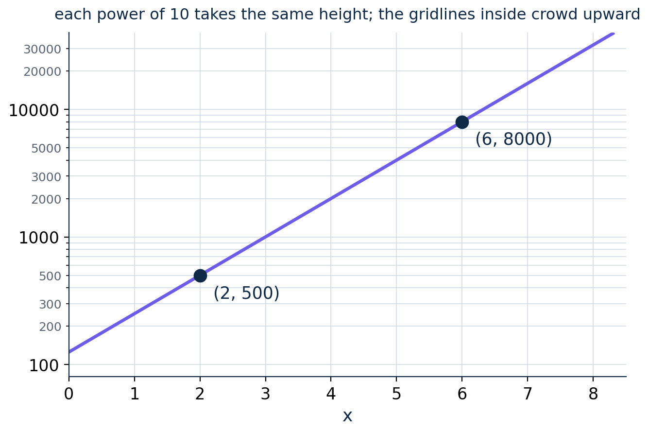
From 100 to 1000 takes the same height as from 1000 to 10000. The line through and is an exponential function.
To read a semi-log axis, think in logs. and , so the band from the 100 line to the 1000 line covers from 2 to 3.
Worked example
Reading the axis. (a) A point is 30% of the way up from the 100 line to the 1000 line. What is its y-value? (b) Where does sit in that band?
- 01
(a) 30% of the way means .
- 02
Undo the log: . The point is at about 200, not at .
- 03
(b) , so 400 sits about 60% of the way up the band. (200 sits at 30.1% and 500 at 69.9%; the gridlines are NOT evenly spaced.)
COMMON MISTAKE
“Halfway between the 100 line and the 1000 line is 550.”
Halfway means , so . The value 550 sits much higher, at . Read heights as powers of 10, not as ordinary distances.
Why Exponential Functions Become Straight
Take log of both sides of and use the product and power rules (2.12):
Compare this with the slope-intercept form of a line, . If we call , the equation is a line with intercept and slope . Plotting against is exactly what a semi-log plot does, so the graph is a straight line. For Nova:
You can see the constant slope in a table: each month adds the same 0.1761 to .
| t (month) | 0 | 1 | 2 | 3 | 4 |
|---|---|---|---|---|---|
| N(t) | 256 | 384 | 576 | 864 | 1296 |
| 2.4082 | 2.5843 | 2.7604 | 2.9365 | 3.1126 |
CONCEPT
Reading the Line
Slope = . A positive slope means growth (); a negative slope means decay (0 < ).
Each 1-unit step in ADDS to , which means MULTIPLYING by . For Nova, +0.1761 in is ×1.5 in .
Intercept = , the value of at . For Nova, .
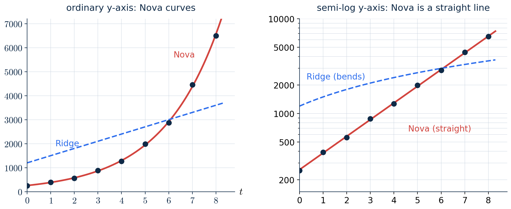
Left: ordinary axes. Right: the same data on a semi-log axis. Nova's points line up; Ridge, which is linear, now BENDS.
Why does Ridge bend? Its log values go 3.0792, 3.1761, 3.2553, … and the differences 0.0969, 0.0792, 0.0669, 0.0580 keep shrinking. Adding a fixed 300 is a SMALLER and smaller factor as the amount grows, so a linear function is concave down on a semi-log plot.
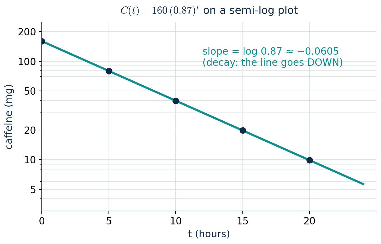
Decay is a straight line too, sloping downward. Every 5 hours the line drops by the same height, because the caffeine is multiplied by the same factor.
KEY RULE
Straight on a semi-log plot ⇔ exponential. Bending ⇔ not exponential.
Quick check
A semi-log line has slope . What is the growth factor ?
Linearizing Data to Build a Model
Nova's actual counts from 2.5B, with a new row, :
| t | 0 | 1 | 2 | 3 | 4 | 5 | 6 | 7 | 8 |
|---|---|---|---|---|---|---|---|---|---|
| y | 250 | 390 | 560 | 880 | 1270 | 1990 | 2870 | 4450 | 6490 |
| 2.398 | 2.591 | 2.748 | 2.944 | 3.104 | 3.299 | 3.458 | 3.648 | 3.812 |
Worked example
Example 1 (by hand). Use two points of the (, ) table to estimate an exponential model for Nova.
- 01
Check linearity: the differences of are all between about 0.16 and 0.20, so (, ) is close to a line. The data is close to exponential.
- 02
Pick two points far apart, and , and find the slope of the line through them:
- 03
Intercept: , so . Estimated model: , which predicts about 6,677 at (actual: 6,490).
Worked example
Example 2 (regression). Use ALL the points to find the best-fitting model.
- 01
Fit a LINEAR regression to the points (, ): . (TI-84: put in L3 and use LinReg on L1, L3. Desmos: add a column and type ~ + c.)
- 02
Undo the log. The slope becomes the base and the intercept becomes :
- 03
Compare: the hand estimate and the regression are close. The regression is better because it uses every point, not just two.
This is exactly the ExpReg model from 2.5B, and that is no coincidence: exponential regression works by fitting a line to the logarithms of the data. That is also where the in 2.5B came from: it measures how straight the (, ) points are. (It's also what Desmos's “Log Mode” does.) With ln instead of log you get and the same and .
COMMON MISTAKE
“The slope is 0.1767, so .”
The slope of the semi-log line is , not . Convert back: . Likewise the intercept 2.4046 is , so , not 2.4046. (If ln was used, convert with instead of 10.)
Quick check
A linear fit gives . Write as an exponential function.
Reading a Model Straight From a Semi-log Graph
Worked example
Example 3. A semi-log plot shows a straight line through and . Find the exponential model .
- 01
The slope of the line is the change in over the change in :
- 02
Or directly: from to , is multiplied by in 4 steps, so and . (The base of an exponential must be positive, so −2 is not possible, as in 2.5A.)
- 03
, so . Check: ✓.
Worked example
Try it yourself. A semi-log line passes through and . Is it growth or decay? Find the model and the slope of the line.
Answer: Decay: the line goes down. , so and . Slope = .
Practice
Worked example
P1. A linearized model is . Write .
Answer: and , so : about 12.2% growth per unit.
Worked example
P2. Caffeine is plotted on a semi-log plot. What are the slope and the intercept of the line (in )?
Answer: Slope (negative: decay) and intercept .
Worked example
P3. On a semi-log plot, data set A lies on a straight line and data set curves downward. Which one is exponential? What might be?
Answer: A is exponential. grows by smaller and smaller factors; it could be linear (like Ridge) or another slower-than-exponential function.
Worked example
P4. A point on a semi-log plot is exactly halfway between the 1000 line and the 10000 line. What is its y-value?
Answer: , so .
Worked example
P5. A semi-log line passes through and . Find its slope and the model.
Answer: Slope = ()/4 ≈ −0.301, so . : .
Common slips
“Halfway between the 100 line and the 1000 line is 550.”
Halfway means , so . The value 550 sits much higher, at . Read heights as powers of 10, not as ordinary distances.
“The slope is 0.1767, so .”
The slope of the semi-log line is , not . Convert back: . Likewise the intercept 2.4046 is , so , not 2.4046. (If ln was used, convert with instead of 10.)
Lock it in
Try the flashcards
6 cards · Semi-log plots and residuals
Recap card
5 lines to re-read the night before.
- 01
A semi-log plot has an ordinary x-axis and a logarithmic y-axis: equal heights are equal factors. Read the axis as powers of 10.
- 02
becomes : a straight line with slope and intercept . Growth slopes up, decay slopes down.
- 03
Straight on a semi-log plot means exponential. A linear function bends (concave down).
- 04
To model data: fit a line to (, ), by two points or by regression; then a = 10^intercept and b = 10^slope. ExpReg does exactly this.
- 05
Unit 2 complete: from Nova's sequence in 2.1 to a straight line in 2.15, adding versus multiplying has been the whole story.